How to Read an Oscilloscope Screen: Understanding Waveforms, from Fundamentals to Advanced Debugging

An Oscilloscope is the fundamental diagnostic instrument in electronics, drawing a graph of an electrical signal to show how voltage changes over time. This real-time visualization helps engineers analyze waveform shape, frequency, and signal integrity to solve complex design and debug challenges.

The Oscilloscope Screen: Your Diagnostic Command Center

The modern oscilloscope remains the crucial tool for anyone working with electronic circuits. Whether you are designing a complex embedded system or simply debugging a power supply, this instrument captures the numerous electrical signals that make a product function.

But simply connecting a probe and seeing a line move is not enough. To effectively master the oscilloscope, you must comprehend the display's terminology, the graticule settings, and the digital acquisition process.

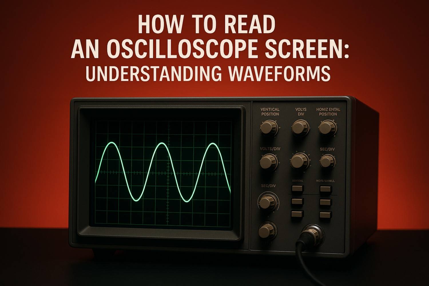
X, Y, and Z: The Three Axes of Waveform Visualization

The core of the oscilloscope display is the graphical representation of an electrical signal over time. The screen, or graticule, organizes this data along three critical axes:

1. X-axis (Horizontal): Time. This is the time base, representing the duration of the signal capture. It is measured in time per division (Sec/div) and is crucial for measuring frequency and period.
2. Y-axis (Vertical): Amplitude. This axis represents the signal’s voltage level. It is measured in volts per division (Volts/div) and defines the maximum voltage of the signal.
3. Z-axis (Intensity): Frequency of Occurrence. In modern Digital Storage Oscilloscopes (DSOs), the intensity or brightness of the trace tells you how often a specific point (e.g., noise or jitter) occurs at a given voltage and time. This insight provides valuable diagnostic information about signal stability that a simple trace cannot.

Understanding Waveform Shape for Immediate Diagnosis

The immediate shape of the signal offers the fastest, high-level troubleshooting feedback.

Waveform Type Description Typical Use/Diagnosis

Sine Wave Smooth, repetitive, alternating between positive and negative peaks. Foundational signals in telecommunications; ideal reference for periodic events.

Square/Pulse Wave Abrupt, instantaneous transitions between low and high states. Digital logic (clock signals, data buses); power control (PWM).

Complex Waveform Signals that require multiple trigonometric functions to describe (e.g., sawtooth, square wave). Motor control, audio/video signals. Distortion here often points to frequency-related issues.

Visual inspection is robust. If your input square wave has "rounded shoulders," that is an immediate, visual indicator that your circuit or measurement system has insufficient bandwidth or excessive capacitance loading. If the signal is noisy, the visual distortion confirms a malfunctioning component or signal integrity failure.

Why Most Basic Settings Fail Junior Engineers

Many beginner errors stem from an incomplete understanding of how the three central control systems Vertical, Horizontal, and Trigger interact with each other. A bad setting in one area can completely invalidate the reading, even if the waveform looks stable. As RevineTech's team knows, solving real-world design challenges requires robust tools and the knowledge to use them correctly.

Vertical System Mastery: Scaling the Voltage (Volts/Div)

The Vertical controls govern the Y-axis. The goal here is simple: maximize your signal's vertical space on the screen.

The vertical scaling control (Volts/div) adjusts the signal’s amplification or attenuation. For the most accurate voltage measurements, you must adapt this scale so the signal covers the maximum possible area of the graticule. Why? By using more physical screen space, you increase the measurement resolution, ensuring that automated cursor measurements or manual readings are as precise as possible.

 

Horizontal System: Time Base, Sampling, and Avoiding Digital Ghosts (Aliasing)

The Horizontal system (Sec/div) sets the time window you are observing. In a Digital Storage Oscilloscope (DSO), this setting is directly tied to the crucial process of digital acquisition.

The DSO digitizes your continuous input signal by taking discrete samples and storing them in memory to form the waveform record.

• The Problem of Aliasing: If the input signal is sampled too slowly, the oscilloscope cannot accurately rebuild the original waveform. Instead, it generates an alias signal—a false, lower-frequency representation of the truth.
• The Nyquist Rule: To prevent this, the Nyquist rule requires sampling at a rate at least twice the highest frequency component of your signal. A safer engineering guideline recommends setting the sample rate to at least 2.5 times the oscilloscope’s specified bandwidth to ensure high-fidelity representation.

Improper adjustment of the time base is not just a visual error; it compromises the integrity of the underlying digital data.

Triggering: The Key to a Stable Picture

The trigger system is indispensable for nearly all oscilloscope operations, as it defines when the oscilloscope begins acquiring data.

1. Stabilization: For repetitive signals, the trigger ensures that each sweep begins at the exact same point on the waveform, giving you a stable, usable display.
2. Event Capture: For non-periodic, transient events (like a one-time glitch), the trigger captures the event reliably within the acquisition time window.

The most common setting is Edge Triggering, where the scope begins recording when the signal crosses a defined voltage threshold, or Trigger Level, on either the rising or falling edge. If you cannot achieve a stable, clean picture, the trigger configuration is the first place to check.

Level 3 Mastery: Quantifying the Waveform (The Core Measurements)

Once you have a stable, non-aliased, and accurately scaled waveform, the next step is to translate that visual data into quantifiable engineering metrics. While cursors and automated functions handle the calculations, you must know what each measurement means for your circuit performance.

Measurement Axis of Reference Insight Gained

Peak-to-Peak Voltage ($V_{p-p}$) Vertical (Y) The total voltage difference between the highest positive peak and the lowest negative peak.

RMS Voltage ($V_{RMS}$) Derived (Math) The Root Mean Square voltage—the adequate, average amplitude used to calculate the power delivered by the signal.

Period ($T$) Horizontal (X) The duration (in seconds) required for one complete repeating cycle of the waveform.

Frequency ($f$) Derived (Math) The reciprocal of the period ($f = 1/T$), measured in Hertz (repetitions per second).

Duty Cycle Horizontal (Time): The percentage of one whole period that a signal remains in its “on” state.

Rise Time Horizontal (Time) The time needed for a signal's voltage to transition from a low level (e.g., 10%) to a high level (e.g., 90%).

Remember, the reliability of these calculated numbers is only as good as the setup for acquisition. If the input data is flawed (e.g., due to aliasing or improper probing), the calculated frequency or rise time will be precise but inaccurate.

This One Advanced Feature Will Save You Days in Debugging

For intermittent, non-periodic problems the ones that cause the most elusive system failures—you need advanced Digital Storage Oscilloscope (DSO) features. Modern DSOs are designed to capture and analyze the subtle anomalies that standard edge triggering misses.

Beyond Simple Edges: Pulse, Logic, and Runt Triggering

If a fault happens once every few hours, waiting for it is a waste of valuable engineering time. Specialized triggering transforms the oscilloscope from a passive display device into an active fault hunter.

• Pulse Width Triggering: This mode is crucial for troubleshooting digital logic. It allows you to set the scope to capture only when a pulse duration is greater than, less than, or not equal to a specified time value. This is perfect for catching timing anomalies.
• Logic Triggering: When debugging complex buses, you may need a trigger defined by a logical combination across multiple channels (e.g., Channel 1 is HIGH and Channel 2 is LOW). Logic triggering enables this complex, conditional capture.
• Runt Triggering: This is a diagnostic hero for signal integrity. A runt pulse is a signal that starts to transition but fails to cross the necessary voltage threshold, signaling severe degradation. Runt pulses are often caused by bus-contention problems, where two components try to drive the same bus line simultaneously. The ability to isolate and trigger on this specific abnormality saves days of guesswork.

Frequency Domain Analysis with FFT

While the time domain (voltage vs. time) is intuitive, many critical faults like power supply noise, EMI, or harmonic distortion—are best analyzed in the frequency domain (amplitude vs. frequency).

The Fast Fourier Transform (FFT) function built into DSOs performs this conversion, allowing you to dissect the signal's spectral purity instantly.

The Link to Memory Depth: The quality of your FFT plot depends on your acquisition settings. The frequency span (the maximum frequency observed) is set by the sampling rate. However, the crucial frequency resolution bandwidth ($\Delta$f)—how closely two frequencies can be distinguished is determined by the total record length (acquisition time). Deep memory depth enables the DSO to maintain a high sample rate over a longer acquisition time, which in turn provides the acceptable frequency resolution necessary to separate closely spaced spectral components, such as system noise, from harmonics.

Probing Physics: Why the Measurement System Can Lie to You

The signal displayed on the screen is only as good as the probe connecting it to your circuit. The probe is the most significant potential source of error because it introduces an electrical load (capacitance and impedance) that can unintentionally alter the circuit's behavior.

Probe Compensation: The Pre-Flight Check

Before taking any meaningful measurement with a passive probe, you must perform probe compensation. This mandatory procedure counterbalances the inherent input capacitance of the oscilloscope.

1. Connect the probe to the scope's built-in reference signal (usually a 1000 Hz square wave generator).
2. Adjust the variable capacitance inside the probe housing (using a non-conductive tool) until the displayed square wave is perfectly rectangular.

If the square wave shows rounded corners (undercompensated) or excessive overshoot/ringing (overcompensated), your probe is introducing distortion, and every subsequent measurement will be invalid.

The 3x Rule for Bandwidth Selection

One of the most common causes of inaccurate digital signal readings is insufficient probe bandwidth. The probe must not limit the measurement system.

Leading experts suggest the probe bandwidth should be at least equal to the oscilloscope's bandwidth. More critically, for accurate measurement of signal edges (Rise and Fall times), the probe bandwidth should be at least three times the highest fundamental frequency of the signal being measured. If you violate this rule, your system cannot accurately capture the necessary high-frequency harmonic components, and the displayed rise time will be artificially slowed, giving you a misleading view of your circuit's performance.

Active vs. Passive Probes: Minimizing Load

To achieve the best signal integrity measurements, you must minimize the probe's loading effect.

• Passive Probes: Cost-effective and robust, but have higher input capacitance, increasing circuit loading, especially at higher frequencies.
• Active Probes: These probes feature internal amplifiers, providing extremely high input impedance and, critically, very low input capacitance (often less than four pF, or even below one pF for premium models). Low capacitance minimizes high-frequency loading, preserving the signal's integrity and providing a faithful representation on the screen.

To ensure confidence in your high-speed designs, you must choose a low-capacitance active probe and use the shortest possible ground leads to minimize induced inductance.

Visualizing System Health with the Eye Diagram

For high-speed digital design, signal integrity (SI) is paramount. The Eye Diagram is the visualization tool of choice, aggregating thousands of digital transitions into one statistical picture.

A wide-open eye means good SI, while a closed or constricted eye indicates excessive jitter, noise, or timing errors. To diagnose SI issues accurately, you must probe the signal as close to the receiver of the Device Under Test (DUT) as physically possible. Probing at the beginning of the transmission line gives an unrepresentative reading; only probing near the receiving component shows the actual, degraded signal that the element actually "sees".

Final and Next Steps for RevineTech Customers

Mastering the oscilloscope screen involves more than simply reading voltage and time; it requires a systematic, multi-layered approach that includes accurate setup, leveraging advanced digital features, and validating the integrity of the physical measurement system.

Why Calibration is Non-Negotiable

The final and most critical layer of trust in your readings is the calibration status of the instrument. Over time, due to usage and environmental factors, an oscilloscope's performance can drift, leading to inaccurate measurements of signal amplitude, frequency, and timing.

Regular calibration ensures that your instrument maintains its specified accuracy, providing the necessary confidence in your data to make informed design decisions. This is not just a technical suggestion; in sectors like medical engineering and aerospace, it is a regulatory requirement for compliance and safety.

Which Oscilloscope is Right for You? (Call to Action)

RevineTech’s mission is to be the technology partner that helps you overcome complex design and debug challenges, enabling faster product development. The best oscilloscope for you is the one that provides the essential features discussed here—deep memory, robust triggering (like Runt), sufficient bandwidth, and support for low-capacitance active probes—at an optimized price point.

Our team of dedicated Application and Product Managers combines engineering expertise with real-world insight to provide personalized solutions tailored to your specific technical needs.

Need to ensure your next product launch is error-free? Contact our experts today to discuss the ideal oscilloscope and probing solution for your high-speed digital design or power electronics application.

Content Refresh Idea: Check back quarterly for updates on new oscilloscope firmware releases, which frequently introduce new triggering modes (such as power analysis triggers) and enhanced math functions (like advanced jitter decomposition), further extending the life and capabilities of your instrument.